Introduction to Classification along with prerequisites

What do you mean by Classification?

The process of recognition, understanding, and grouping of objects and ideas into preset categories. In simple terms, it can be understood as a form of “pattern recognition,”.

Classification algorithms used in machine learning utilize input training data for the purpose of predicting the likelihood or probability that the data that follows will fall into one of the predetermined categories.

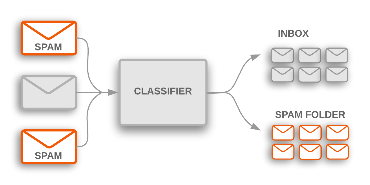
For example, we might decide if an email is spam, if it exceeds spam probability of 0.7. That 0.7 is our classification threshold. If an email has a spam probability over 0.7 probability then its spam otherwise not.

A.Binary Classification: we have only two class labels.

For example our spam email classification, either our email is spam or not spam depending on our value of classification threshold.

B.Multi class Classification: we have more than two class labels.

For example our IRIS classification, either our flower is setosa or versicolor or virginca depending.

Different types of classification algorithms are,

1.Logistic Regression:

We use logistic regression for the binary classification of data-points. We perform categorical classification such that an output belongs to either of the two classes (1 or 0). 

For example – Spam email classification, it is either spam or not spam.

Two of the important parts of logistic regression are Hypothesis and Sigmoid Curve. With the help of this hypothesis, we can derive the likelihood of the event. The data generated from this hypothesis can fit into the log function that creates an S-shaped curve known as “sigmoid”. 

h = g(K^(t) * X), where g is the sigmoid function, 

g(w) = 1 / (1 + e^(-w))

After substituting g in h, we get

h = 1 / (1 + e^(-Kt) * X)

where,

1. h(x) is interpreted as the probability that y = 1 for input x
2. X is probability of events such as that some email message x is spam (1) as opposed to ham (0)
3. w is a set of parameters. Different values for the parameters w lead to different decision boundaries

We can use Gradient Descent to find the values of w that have the lowest cost

Logistic regression has some commonalities with linear regression, but you should think of it as classification, not regression.

Advantages of Logistic regression,

1. They are super easy to implement.
2. The probabilities resulting from this approach are well-calibrated. This makes it more reliable than other models.
3. They are less prone to over-fitting by using a technique referred to as regularization.
4. It provides a more accurate result for many simple data sets than when any other approach is used. It, however, performs well when the data set has linearly separable features.
5. Logistic regression can easily extend to multiple classes and a natural probabilistic.

Disadvantages of logistic regression,

1. High dimensional datasets lead to the model being over-fit, leading to inaccurate results on the test set. As very high regularization may result in under-fit on the model, resulting in inaccurate results.
2. Non-linear problems cannot be solved using the logistic regression technique.
3. Logistic regression is not as powerful as other algorithms.
4. When the number of observations is lesser, it may result in over-fitting.
5. In logistic regression, data maintenance is higher as data preparation is tedious.

2.K-Nearest Neighbors(KNN):

K-Nearest Neighbour (K-NN) is a simple algorithm that stores all the available cases and classifies the new data or case based on a similarity measure. It queries the k points that are closest to the sample point and returns the most frequently used label of their class as the predicted label.

For example- IRIS flower Classification into Virginica, Versicolor or Setosa.

It is called Lazy algorithm because it does not need any training data points for model generation. As, all training data is used in the testing phase which makes training faster and testing phase slower and costlier.

How to choose K?

k is a free “hyperparameter” of the algorithm.

1. One option is to try different values of k when evaluating on test data.
2. Rather than split data into two parts, training and test, we split data into three parts, training and validation (aka development) and test.
3. Use the validation data as “pseudo-test data” to tune (choose best) k○Do final evaluation on the test data only once

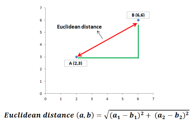
How do we calculate the distance between various class labels?

The Euclidean distance is the most common distance metric used in low dimensional data sets.While Euclidean distance is useful in low dimensions, it doesn’t work well in high dimensions and for categorical variables. 

The drawback of Euclidean distance is that it ignores the similarity between attributes.

Advantages of KNN

1. Simple and intuitive
2. Data does not have to be linearly separable

Disadvantages of KNN:

1. Need to store large full training data
2. Test time is very slow
3. Prefer to pay for expensive training in exchange for fast prediction
4. kNN is an instance-based classifier: must carry around training data (waste of space)
5. Training easy yet Testing hard

3.Decision Tree:

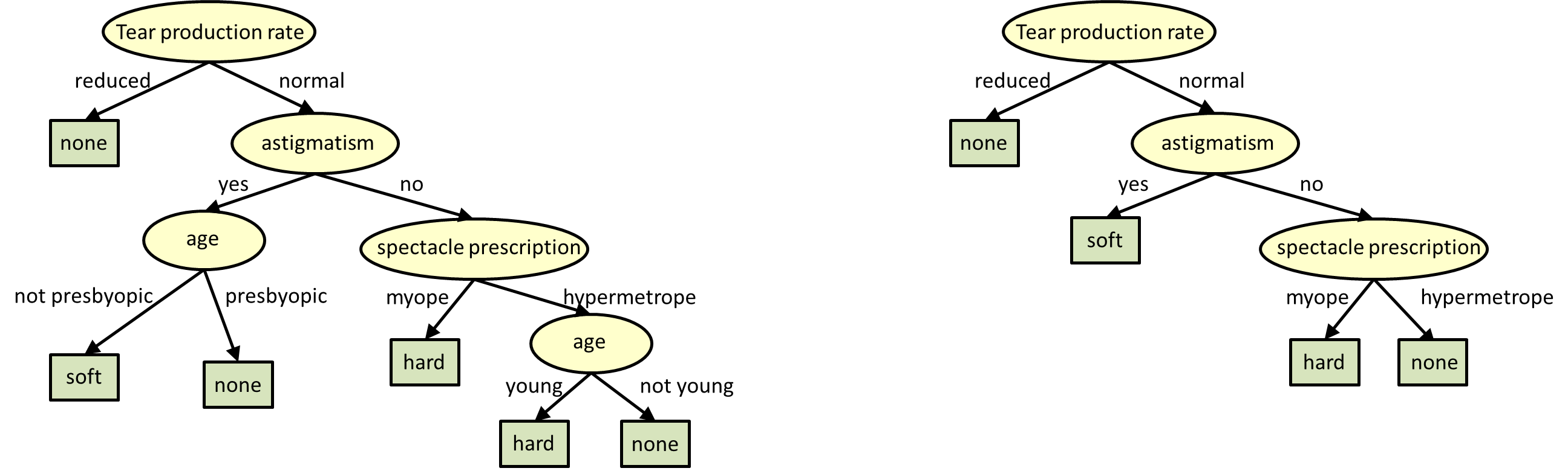
A decision tree represents a procedure for classifying categorical data based on their attributes. The construction of decision tree does not require any domain knowledge or parameter setting and there for appropriate for exploratory knowledge discover.

The tree should be compact, so that it generalizes well to non-training data without overfitting and it should predict labels of training data accurately.

A decision tree has 2 kinds of nodes,

1. Each leaf node has a class label, determined by majority vote of training examples reaching that leaf.
2. Each internal node is a question on features. It branches out according to the answers.

What do you mean by Entropy and Information Gain?

Entropy is a measure of uncertainty or impurity. More uncertainty, more entropy!

The information gain when we divide the data using a particular feature is the reduction in entropy.

When deciding what feature to test at the root of a tree, we look at the entropy at the root node (parent) and the entropy at the children of the root node.

Using different features at the root to split the data will result in different children with different entropies. We greedily choose the feature that maximizes information gain

Information Gain = entropy(parent) - [weighted average entropy(children)]

What about over fitting?

On some problems, a large tree will be constructed when there is actually no pattern to be found. Over fitting becomes more likely as the hypothesis space and the number of inputs grows, and less likely as we increase the number of training examples

Decision trees will over fit as standard decision trees have no learning bias and lots of variance. We must introduce some bias towards simpler trees

How to Build Small Trees?

1. If growing the tree larger hurts performance, then stop growing
   1. Fixed depth
   2. Fixed number of leaves
2. Grow the full tree, then prune the tree bottom-­‐up (collapse some sub trees)

Advantages of Decision tree,

1. Easy to understand how to implement
2. Work well in practice for many problems
3. Easy to explain model predictions, i.e., interpretable

Disadvantages of Decision tree,

1. Need to store large tree
2. No principled pruning method to avoid overfitting
3. Not effective for all problems, e.g., the majority function, which returns 1 if and only if more than half the inputs are 1, and returns 0 otherwise (requires an exponentially large decision tree)

4.Various Ensemble Methods

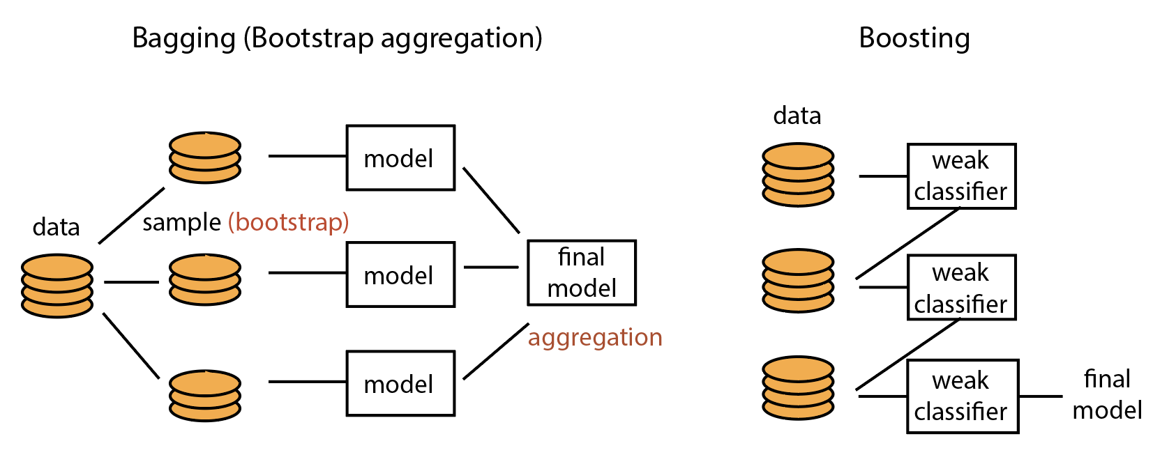
Ensemble methods combine several base models in order to produce one optimal predictive model

Rather than just relying on one Decision Tree and hoping we made the right decision at each split, Ensemble Methods allow us to take a sample of Decision Trees into account, calculate which features to use or questions to ask at each split, and make a final predictor based on the aggregated results of the sampled Decision Trees.

1. Bagging: Take repeated samples from the training set to generate many different bootstrapped training sets. Construct a tree for each bootstrapped training set, creating a collection of trees. To make a prediction for a new example, take the majority classification prediction from the bagged collection of trees.
2. Boosting: Trees are learned sequentially. Consecutive trees are based on the error from the previous tree. When an input is miss classified by a tree, its weight is increased so that the next tree is more likely to classify it correctly. Trees are kept small so that the boosting approach learns slowly. With each subsequent tree, we improve the fit in areas where the previous tree did not perform well.

3.Random Forest: As with bagging, a collection of trees is created from bootstrapped training samples. With random forests, however, each time we construct a node in a tree by choosing greedily among the features, we choose among all features but rather among a randomly sampled subset of features.

How are we going to evaluate the quality of that model, after choosing classification method?

We need some new metrics, our regression metrics aren’t sufficient. These metrics depend on our data set types,

For all these metrics we consider a matrix of 2 * 2 dimension, containing all the outcomes. For example, we can consider a model categorizing an apple from a data set containing apples and oranges.

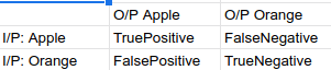
1. True Positive: Input is an apple and output is an apple
2. False Negative: Input is an apple and output is an orange
3. False Positive: Input is an orange and output is an apple
4. True Negative: Input is an orange and output is an orange

Various metrics we use are

1.Precision: Ratio of Correct Predictions by total predictions

Precision (H) = TP /(TP+FP)

2.Recall: Ratio of Correct Predictions by total Items

Recall (H) = TP /(TP+FN)

Whenever someone tells you what the precision value is, you need to also ask about the recall value before you can say anything about how good the model is.

3.Accuracy: Ratio of number of correct predictions divided by the total number of predictions

Accuracy = (TruePositive + TrueNegative) / Total

4.F1 Score: It is the harmonic mean of precision and recall

F1-score = 2*Precision*Recall / (Precision+Recall)

Q.When to use accuracy and when to use other metrics?

We usually use Accuracy only for balanced data sets, i.e datasets containing the same number of items from all the classes

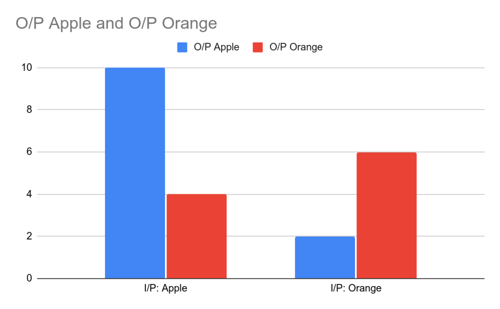
So for example of apples and oranges,

Accuracy for model is: (I/P Apples and O/ P Apple + I/P Oranges and O/P Oranges) / Sum of all values in matrix.
Accuracy for model = 10/20 = 50 %

We usually use F1 Score for Unbalanced data sets i.e datasets not containing the same number of items from all the classes.

F1 score for model is: (Recall + precision) /2
Recall= TP /(TP+FN) = 10/ 14 = 0.714
Precision = TP /(TP+FP)= 10/ 12 =0.833
F1 score = 0.7735 %

For more information,

1. https://www.cs.toronto.edu/~urtasun/courses/CSC411_Fall16/CSC411_Fall16.html
2. https://people.csail.mit.edu/dsontag/courses/ml12/
3. https://www.autonlab.org/resources/tutorials

Previous blog was related to regression : https://programmerprodigy.code.blog/2021/05/15/introduction-to-regression-along-with-prerequisites/

My GitHub repository: https://github.com/kakabisht/AI_lab