Introduction to Regression along with prerequisites

Simple Linear Regression

Linear regression is a statistical model that examines the linear relationship between two or more variables a dependent variable and independent variable(s).

Linear relationship basically means that when one (or more) independent variables increases (or decreases), the dependent variable increases (or decreases) too.

Simple Linear Regression predicts Y on the basis of a single Predictor variable X. It assumes that there is a linear relationship between X and Y

 y = θ0+ θ1.X, where θ0 = Intercept at Y and θ1 = slope.

1. θ0  and θ1 are known as model coefficients or parameters
2. θ0  is the expected value of Y when X=0.
3. Θ1 is the average increase in Y as per one unit increase in X. 

Fitting Simple Linear Regression?

We fit  Linear  Regression model using training data and estimate model coefficients θ0 and θ1. We can predict future ŷ for the particular x as

1. Y-hat ŷ  = θ0 + θ1.X
2. ŷ indicates prediction of Y on the basis of X=x

The most common approach of measuring closeness involves minimizing the least squares criterion.

Ordinary  Least  Square ?

Ordinary Least Squares is a method in Linear Regression for estimating the unknown parameters by creating a model which will minimize the sum of the squared errors between the observed data and the predicted one.

It works by making the total of the square of the errors as small as possible (that is why it is called “least squares”). So, when we square each of those errors and add them all up, the total is as small as possible.

What do you mean by Hypothesis and Cost Function?

1.Hypothesis here represents probability of observing an outcome. We want a hypothesis that is bounded between zero and one, regression hypothesis line extends beyond this limits.

1. h (hypothesis): A single hypothesis, e.g. an instance or specific candidate model that maps inputs to outputs and can be evaluated and used to make predictions.
2. H (hypothesis set): A space of possible hypotheses for mapping inputs to outputs that can be searched, often constrained by the choice of the framing of the problem, the choice of model and the choice of model configuration.

2.Cost function: There’s a hypothesis function to be found. More precisely we have to find the parameters θ0 and θ1 so that the hypothesis function best fits the training data. By tweaking θ0 and θ1 we want to find a line that represents at best our data.

We need a function that will minimize the parameters over our data set. One common function that is often used is mean squared error, which measure the difference between the estimator (the data set) and the estimated value (the prediction).

To understand the math behind cost function ,

1. https://www.coursera.org/lecture/machine-learning/cost-function-rkTp3

What do you mean by Gradient descent?

Let’s say you are at top of a hill and you want to reach the bottom of the hill. You have two options to reach the bottom or minima of the hill. You could either,

1. Take small steps and cover small distance per step. This will ensure we reach the bottom, it might be time consuming but it guarantees reaching the bottom.
2. Take a snowboard and cover large distances. This will ensure that you are really quick but it might make you miss the bottom and go further away from the bottom.

θj+1 := θj − α ∂/∂θj (J(θ)) where, 
θj is the old position
θj+1 is the new position
α is the learning rate
∂/∂θj (J(θ)) is the gradient of function J for θj

Depending on the amount of data, we make a trade-off between the accuracy of the parameter update and the time it takes to perform an update.

1. Batch Gradient Descent: It processes all the training examples for each iteration of gradient descent. But if the number of training examples is large, then batch gradient descent is computationally very expensive.
2. Stochastic Gradient Descent: It processes 1 training example per iteration. Hence, the parameters are being updated after one iteration in which a single example has been processed. Hence it’s quite faster than batch gradient descent. But again, when the number of training examples is large, even then it processes only one example which can be additional overhead for the system as the number of iterations will be quite large.
3. Mini Batch gradient descent: It works faster than both batch gradient descent and stochastic gradient descent. If the number of training examples is large, it is processed in batches of b training examples in one go. Thus, it works for larger training examples and that too with lesser number of iterations.

For gradient descent, the learning rate( size of steps ) is a hyper parameter. A parameter that is set before the learning process begins. These parameters are set in order to find ideal values of parameters, where we minimize the least squares error.

A model converges when additional training will not improve the model. Gradient descent can converge to local minimum, event with the learning rate Alpha fixed. As we approach a local minimum , gradient descent will automatically take smaller steps. So, no need to decrease alpha over time.

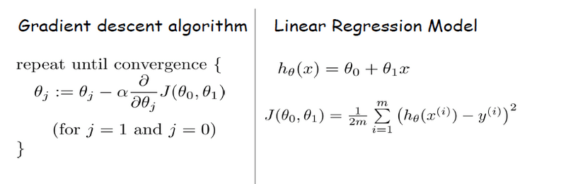
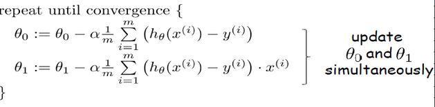
If we substitute equation of linear regression into gradient descent algorithm, we could find the local minimum in the model. The equation should look similar to this,

Categorical Data?

Our Machine Learning Algorithms can’t process categorical data, so how should we handle categorical data?

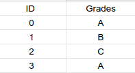
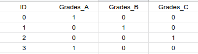
We use a variety of encoding algorithms, let us consider this data set for an example

Let us consider how we will, use two algorithms to make categorical data work in regression

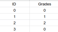
1.Label Encoding

1. Take the unique values from categorical column and store them in a list.
2. Sort list in ascending order.
3. Replace the values of unique values in categorical column by their index positions in the list.

Hence A=0,B=1 and C=1

2.One hot Encoding

1. Take the unique values from categorical column.
2. Create a column for each unique categorical column

Multiple and Polynomial Linear regression?

Multiple linear regression is used to estimate the relationship between two or more independent variables and one dependent variable. You can use multiple linear regression when you want to know.

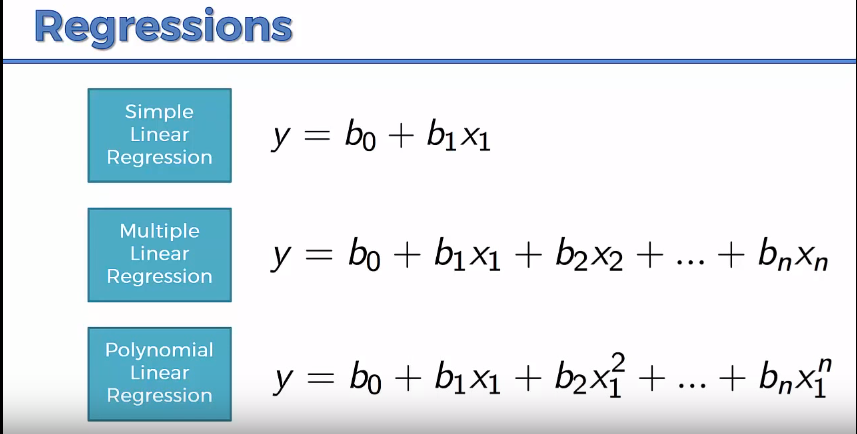
Where y = the predicted value of the dependent variable, b0 = Intercept at Y and bn = the regression coefficient (bn) of the nth independent variable (Xn) 

We have to find the degree of polynomial that fits our requirements if we choose a low degree of polynomial we might face under fitting but if we choose a high degree of polynomial we might face over fitting. So, we have to look for the correct power to generate a generalized model.

How to solve the problem of over fitting(Regularization)?

The model will have a low accuracy if it is overfitting. This happens because your model is trying too hard to capture the noise in your training dataset.

Ridge regression discourages learning a more complex or flexible model, so as to avoid the risk of over fitting. If there is noise in the training data, then the estimated coefficients won’t generalize well to the future data. This is where regularization comes in and shrinks or regularizes these learned estimates towards zero.

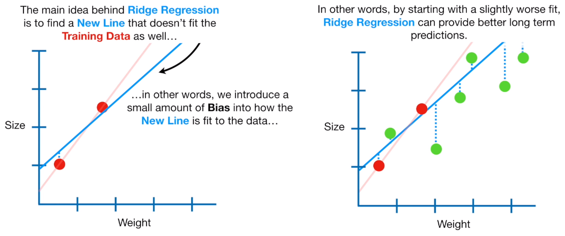
It is a useful technique that can help in improving the accuracy of your regression models. Another example is Lasso regression.

For more information ,

1. https://medium.com/swlh/gradient-descent-algorithm-3d3ba3823fd4
2. https://online.stat.psu.edu/stat462/node/91/
3. https://www.machinecurve.com/index.php/2020/11/02/machine-learning-error-bias-variance-and-irreducible-error-with-python/
4. https://www.simplilearn.com/tutorials/machine-learning-tutorial/regularization-in-machine-learning

GitHub repository containing the code: https://github.com/kakabisht/AI_lab