Basics of Statistics and Data Analysis

AI is likely to be either the best or the worst thing to happen to humanity.

Stephan Hawking

I took Introduction to Artificial Intelligence class at my university given by Swati Ahirao ma’am. This blog covers the basics of Statistics and data analysis required for Artificial Intelligence.

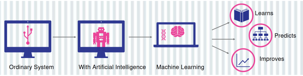
What do you mean by Artificial Intelligence?

Intelligence is the ability to learn from the environment and change our behavior based on inputs we get. Simulation of human intelligence in machines that are programmed to think like humans and mimic their actions.

We make the machines copy or perform the cognitive functions that we associate with human minds such as problem solving, learning and decision making.

What do you mean by Machine Learning?

Machine Learning is the application of Artificial Intelligence(AI) that provides systems the ability to automatically learn and improve from experience without being explicitly programmed.

Basic Statistics and Exploratory Data Analysis

  1.Descriptive Statistics:

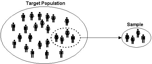
1. Population :- Collections of all items of interest to our study and usually denoted with N.
2. Sample :-  Subset of Population and usually denoted with n.

A random sample is collected when each member of the sample is chosen from the population strictly by chance. A representative sample is a subset of the population that accurately reflects the members of the entire population.

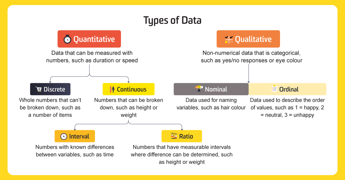
Types of data,

1.Quantitative data  represents  number.  It is divided into two groups: 

1. Discrete data can be usually counted in a finite matter.
2. Continuous data is infinite, impossible to count, and impossible to imagine.

2.Qualitative data represents categorical values. It is further divided into nominal and ordinal 

1. Nominal variables are categories like car brands – Mercedes, BMW or Audi, or like the four seasons – winter, spring, summer and autumn. They aren’t numbers and cannot be ordered.
2. Ordinal data, on the other hand, consists of groups and categories which follow a strict order

As a general rule, counts are discrete and measurements are continuous.

1. Quantitative data are measures of values or counts and are expressed as numbers. Quantitative data are data about numeric variables (e.g. how many; how much; or how often).
2. Qualitative data are measures of ‘types’ and may be represented by a name, symbol, or a number code. Qualitative data are data about categorical variables (e.g. what type).

Common methodologies used in data analysis,

1.Mean: The “average” number; found by adding all data points and dividing by the number of data points.

     For Ex. The mean of 4, 1, 7  is  4 

2.Median: The middle number; found by ordering all data points and picking out the one in the middle (or if there are two middle numbers, taking the mean of those two numbers). 

    The order of number here is  1,4,7

     For Ex.  The median  is  4 

3.Mode: The most frequent number—that is, the number that occurs the highest number of times.

     For Ex.  {4, 2, 4, 3, 2, 2}   The mode is  2

4.Variance: It measures the dispersion of a set of data points around their mean.

5.The standard deviation of a data set is a measure of the magnitude of deviations between the values of the observations contained in the data set.

Variance gives results in squared units. Standard Deviation is the most common measure of variability for a single data set .

6.The coefficient of variation (relative standard deviation) is a statistical measure of the dispersion of data points around the mean.

Unlike the standard deviation that must always be considered in the context of the mean of the data, the coefficient of variation provides a relatively simple and quick tool to compare different data series. The advantages of the Co-efficient of Variation are,

1. Doesn’t have a unit of measurement
2. Universal across datasets
3. Perfect for comparisons

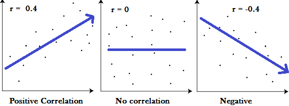
How is the correlation coefficient used?

The correlation coefficient is the specific measure that quantifies the strength of the linear relationship between two variables in a correlation analysis. The coefficient is what we symbolize with the r in a correlation report.

For two variables, the formula compares the distance of each data point from the variable mean and uses this to tell us how closely the relationship between the variables can be fit to an imaginary line drawn through the data.

What are some limitations to consider?

Correlation only looks at the two variables at hand and won’t give insight into relationships beyond the bivariate data. This test won’t detect (and therefore will be skewed by) outliers in the data and can’t properly detect curvilinear relationships.

2.Inferential  Statistics

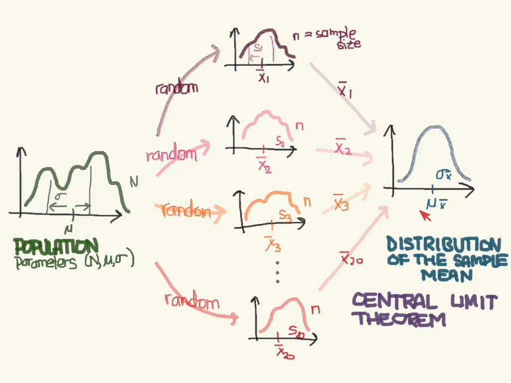
Central  Limit  Theorem:

The central limit theorem states that if you have a population with mean μ and standard deviation σ and take sufficiently large random samples from the population with replacement, then the distribution of the sample means will be approximately normally distributed.

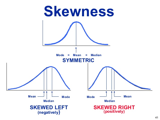
1.Symmetric Distribution: A symmetric distribution is a type of distribution where the left side of the distribution mirrors the right side.

Distributions don’t have to be unimodal to be symmetric. They can be bimodal (two peaks) or multimodal (many peaks).

 2.Skewed  Distribution:

1. A left-skewed distribution has a long left tail. Left-skewed distributions are also called negatively-skewed distributions. That’s because there is a long tail in the negative direction on the number line. The mean is also to the left of the peak.
2. A right-skewed distribution has a long right tail. Right-skewed distributions are also called positive-skew distributions. That’s because there is a long tail in the positive direction on the number line. The mean is also to the right of the peak.

Long tails mean there are Outliers (data points that are far from other data points) in the data set. To know more about removing Outliers,

1. https://statisticsbyjim.com/basics/outliers/

What is sampling ?

1.Simple random sample: Every member and set of members has an equal chance of being included in the sample. Technology, random number generators, or some other sort of chance process is needed to get a simple random sample.

• Example—A teachers puts students’ names in a hat and chooses without looking to get a sample of students.
• Random samples are usually fairly representative since they don’t favor certain members.

2.Stratified random sampling: The population is first split into groups. The overall sample consists of some members from every group. The members from each group are chosen randomly.

• Example—A student council surveys 100 students by getting random samples of 25 freshmen, 25 sophomores, 25 juniors, and 25 seniors.
• A stratified sample guarantees that members from each group will be represented in the sample, so this sampling method is good when we want some members from every group.

 3.Interval Sampling: interval sampling. E. g.  pick up item after every 10

Types of Inferences ?

1.The point estimate is the statistic calculated from sample data used to   estimate the true unknown value in the population called the parameter.

A point estimate of a population parameter is a single value used to estimate the population parameter. For example, the sample mean x is a point estimate of the population mean μ.

Whereas, a confidence interval, naturally, is an interval.

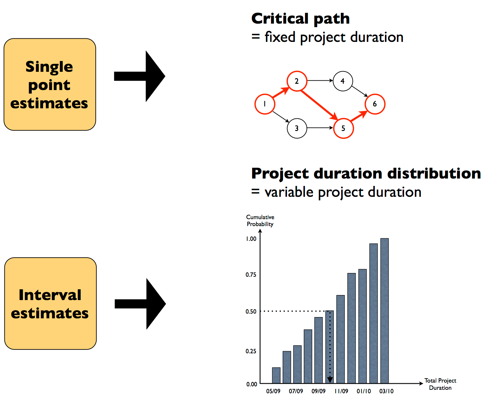
2. An Interval Estimate: An interval is a range of values for a statistic. For example, you might think that the mean of a data set falls somewhere between 10 and 100 (10 < μ < 100). A related term is a point estimate, which is an exact value, like μ = 55.

3.Inter-Quartile Range (IQR): When an ordered data set is divided into four parts, the boundaries are called quartiles. If the same data is divided into 100 parts, each part is called a percentile.

We use 1.5 * IQR rule to detect the Outliers (data points that are far from other data points) in the data set. It is also called 5 number summary.

  3.Exploratory  Data  Analysis

A technique to evaluate predictive models by partitioning the original sample into a training set to train the model, and a testing set to evaluate it. Splitting of data sets

1. Training Set: Used for making the algorithm learn.
2. Testing Set:Used to give input to the algorithm and check against the actual output.

Three Types of analysis,

1. Univariate analysis: the examination of the distribution of cases on only one variable at a time.(eg., college graduation)
2. Bivariate analysis: the examination of two variables simultaneously (e.g., the relation between gender and college graduation)
3. Multivariate analysis: the examination of more than two variables simultaneously (e.g., the relationship between gender, race, and college graduation)

For more information on Basic Statistics and Exploratory Data Analysis,

1. https://statisticsbyjim.com/
2. https://www.khanacademy.org/math/statistics-probability/