Basics of an Algorithm and Different Algorithmic Approaches

Backtracking

Backtracking is an approach to solving constraint-satisfaction problems without trying all possibilities.

Backtracking consists of doing a DFS of the state space tree, checking whether each node is promising and if the node is non promising backtracking to the node’s parent.

Suppose you have to make a series of decisions,among various choices, where

You don’t have enough information to know what to choose
Each decision leads to a new set of choices
Some sequence of choices (possibly more than one) may be a solution to your problem

Back tracking is a methodical way of trying out various sequences of decisions, until you find one that “works”

Backtracking is easily implemented with recursion because:

The run-time stack takes care of keeping track of the choices that got us to a given point.
Upon failure we can get to the previous choice simply by returning a failure code from the recursive call

An real life example of this would be Solving a maze,

Given a maze, find a path from start to finish
At each intersection, you have to decide between three or fewer choices:
1. Go straight
2. Go left
3. Go right
You don’t have enough information to choose correctly
Each choice leads to another set of choices
One or more sequences of choices may (or may not)lead to a solution
Many types of maze problem can be solved with backtracking

Each of the problems above are in the some sense the same problem. They all work by calling some initialization function, then for each possible slot, you try each possible value in turn, stopping when a solution is found, or backtracking when we can’t fill the current slot.

Iterative Implementations

The solutions above used recursion to implement backtracking. This is great because if we ever have to backtrack, we return right in the middle of a for-loop so we know the next value to try. This is actually awesome.

Can we do things iteratively?

Well, yeah, but we have to some incrementing an decrementing manually, and some ugly loop controlling.

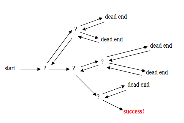
The backtracking algorithm

Backtracking is really quite simple–we“explore” each node, as follows:

To “explore” node N:

If N is a goal node, return “success”
If N is a leaf node, return “failure”
For each child C of N,
1. Explore C
  1. If C was successful, return “success”
Return “failure”

It is convenient to implement this kind of processing by constructing a tree of choices being made called the “State Space Tree”. Its root represents an initial state before the search for the solution begins. The nodes of the first level in the tree represent the choices for the first component of a solution and the nodes of a second level represent the choices for the second component and so on.

A node in the state space tree is promising if it corresponds to the partials constructed solution that may lead to the complete solution otherwise the nodes are called non-promising. Leaves of the tree represent either the non- promising dead end or complete solution found by the algorithm.

Application of Backtracking method:

An application of Back tracking Algorithm is the N Queen Problem:

Given: n-queens and an nxn chess board

Find: A way to place all n queens on the board s.t. no queens are attacking another queen

Let us consider 4 queens as of now, in a chess board. A queen can move,

Horizontal
Vertical
Diagonal

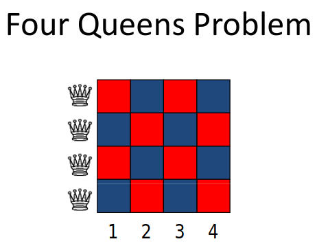
Algorithm for N queens problem:

Now we can place the first queen with out any problems
Before placing the second queen. we will have to check if it does not violate any one condition, i.e not present in the same row, column or diagonal as the first queen.
If we get stuck at a point, after which there is no solution. Then we backtrack to one step before and take an another approach.
We repeat this until we get a solution.

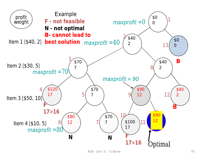
An application of Back tracking Algorithm is the knapsack problem

The profit density of each item (weight / profit) is first calculated, and the knapsack is filled in order of decreasing profit density. A bounding function is used to determine the upper bound on the profit achievable with the current knapsack so as to reduce the search space.

The profit density of each item (weight / profit) is calculated
Filled in order of decreasing profit density.
A bounding function is used to determine the upper bound on the profit achievable with the current knapsack so as to reduce the search space.
Continue until the sack is full

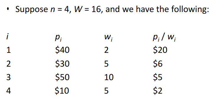
Bounding function is needed to help kill some live nodes without actually expanding them.
A good bounding function for this problem is obtained by using an upper bound on the value of the best feasible solution obtainable by expanding the given live node and any of its descendants. If this upper bound is not higher than the value of the best solution determined so far then that live node may be killed.

More applications of Dynamic programming are,

Subset Sum
Graph coloring
Hamiltonian Cycle

For more information,

Branch and bound

Branch and Bound is a state space search method in which all the children of a node are generated before expanding any of its children.

It is similar to backtracking technique but uses BFS like search.

The different types (FIFO, LIFO, LC) define different ‘strategies’ to explore the search space and generate branches.

1.FIFO (first in, first out): always the oldest node in the queue is used to extend the branch. This leads to a breadth-first search, where all nodes at depth d are visited first, before any nodes at depth d+1 are visited.

2.LIFO (last in, first out): always the youngest node in the queue is used to extend the branch. This leads to a depth-first search, where the branch is extended through every 1st child discovered at a certain depth, until a leaf node is reached.

3.LC (lowest cost): the branch is extended by the node which adds the lowest additional costs, according to a given cost function. The strategy of traversing the search space is therefore defined by the cost function.

Branch and bound keeps a list of live nodes. Four strategies are used to manage the list:

Depth first search: As soon as child of current E-node is generated, the child becomes the new E-node
1. Parent becomes E-node only after child’s subtree is explored
In the other 3 strategies, the E-node remains the E-node until it is dead. Its children are managed by:
1. Breadth first search: Children are put in queue
2. D-search: Children are put on stack
3. Least cost search: Children are put on heap
We use bounding functions (upper and lower bounds) to kill live nodes without generating all their children.

Both BFS and DFS generalize to branch-and-bound strategies

BFS is an FIFO search in terms of live node
1. List of live nodes is a queue
DFS is an LIFO search in terms of live nodes
1. List of live nodes is a stack

Just like backtracking, we will use bounding functions to avoid generating subtrees that do not contain an answer node

An application of Back tracking Algorithm is the knapsack problem

Numbers inside a node are profit and weight at that node, based on decisions from root to that node
Nodes without numbers inside have same values as their parent
Numbers outside the node are upper bound calculated by greedy algorithm
1. Upper bound for every feasible left child (xi=1) is same as its parent’s bound
2. Chain of left children in tree is same as greedy solution at that point in the tree
3. We only recompute the upper bound when we can’t move to a feasible left child
Final profit and final weight (lower bound) are updated at each leaf node reached by algorithm
1. Solution improves at each leaf node reached
2. No further leaf nodes reached after, because lower bound (optimal value) is sufficient to prune all other tree branches before leaf is reached
By using floor of upper bound at nodes, we avoid generating the tree below either node
1. Since optimal solution must be integer, we can truncate upper bounds
2. By truncating bounds at Nodes we avoid exploring Nodes.

An application of Back tracking Algorithm is the Traveling salesman

Definition: Find a tour of minimum cost starting from a node S going through other nodes only once and returning to the starting point S.

Definitions:

A row(column) is said to be reduced iff it contains at least one zero and all remaining entries are non-negative.
A matrix is reduced iff every row and column is reduced.

Branching:

Each node splits the remaining solutions into two groups: those that include a particular edge and those that exclude that edge
Each node has a lower bound.,

Bounding: How to compute the cost of each node?

Subtract of a constant from any row and any column does not change the optimal solution (The path).
The cost of the path changes but not the path itself.
Let A be the cost matrix of a G=(V,E).
The cost of each node in the search tree is computed as follows:
1. Let R be a node in the tree and A(R) its reduced matrix
2. The cost of the child (R), S:
  1. Set row i and column j to infinity
  2. Set A(j,1) to infinity
  3. Reduced S and let RCL be the reduced cost.
  4. C(S) = C(R) + RCL+A(i,j)
Get the reduced matrix A’ of A and let L be the value subtracted from A.
L: represents the lower bound of the path solution
The cost of the path is exactly reduced by L

What to determine the branching edge?

The rule favors a solution through left subtree rather than right subtree, i.e., the matrix is reduced by a dimension.
Note that the right subtree only sets the branching edge to infinity.
Pick the edge that causes the greatest increase in the lower bound of the right subtree, i.e., the lower bound of the root of the right subtree is greater.

For more information,

Difference between Backtracking and Branch and Bound

NP – Hard and NP Complete Problems:

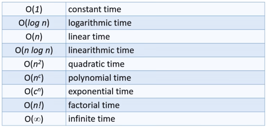
1.Polynomial Algorithms(P):

P is the class of decision problems which can be solved in polynomial time by a deterministic Turing machine. If a problem belongs to P, then there exists at least one algorithm that can solve it from scratch in polynomial time.

Many algorithms complete in polynomial time:

All basic mathematical operations; addition, subtraction, division, multiplication
Linear and Binary Search Algorithms for a given set of number

2.Nondeterministic Polynomial(NP) :

NP is the class of decision problems which can be solved in polynomial time by a non-deterministic Turing machine. Equivalently, it is the class of problems which can be verified in polynomial time by a deterministic Turing machine.

They cannot be solved in polynomial time. However, they can be verified in polynomial time.

3.Nondeterministic Polynomial Hard(NP-Hard) :

NP-hard is the class of decision problems to which all problems in NP can be reduced to in polynomial time by a deterministic Turing machine.

They are not only hard to solve but are hard to verify as well. In fact, some of these problems aren’t even decidable. Some of them are,

Traveling Salesman Problem, and
Graph Coloring

4.Nondeterministic Polynomial Complete(NP-Complete) :

NP-Complete is the intersection of NP-hard and NP. Equivalently, NP-complete is the class of decision problems in NP to which all other problems in NP can be reduced to in polynomial time by a deterministic Turing machine.

For any $\mathcal{NP}$ problem that’s complete, there exists a polynomial-time algorithm that can transform the problem into any other $\mathcal{NP}$ -complete problem. This transformation requirement is also called reduction.

As stated already, there are numerous $\mathcal{NP}$ problems proven to be complete. Among them are:

Traveling Salesman
Knapsack,
Graph Coloring

Curiously, what they have in common, aside from being in $\mathcal{NP}$ , is that each can be reduced into the other in polynomial time. These facts together place them in $\mathcal{NP}\text{-}Complete$ .

For more information,

The GitHub repository for the code are,

If you want to understand basics of graphs, then

https://programmerprodigy.code.blog/2020/10/22/basics-of-graphs/https://programmerprodigy.code.blog/2020/10/22/basics-of-graphs/

Pages: 1 2 3

Basics of an Algorithm and Different Algorithmic Approaches