Basics of an Algorithm and Different Algorithmic Approaches

The information in this blog contains,

1. Page 1: What do you mean by an Algorithm, Time complexity, Space complexity, Orders of growth, Asymptotic Notations, Approach to solve recursive and non recursive algorithms.
2. Page 2: Divide and Conquer, Applications of Divide and Conquer, Greedy Method, Applications of Greedy Method, Dynamic Method, Principle of Optimality and Applications of Dynamic Method.
3. Page 3: Backtracking Method, Applications of Backtracking, Branch and Bound, Applications of Branch and bound, NP Complete and NP Hard problems, GitHub repository with the code .

Introduction:

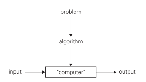
An algorithm is a set of instructions that produces an output or a result. 

It tells the system what to do in order to achieve the desired result. It may not know what the result is beforehand, but it knows that it wants one.

An example for an algorithm, will be cooking a cake. We have our desired output which is a cake, now we have to follow certain set of instructions to make a cake.

There are two kinds of efficiency:

1. Time Efficiency/Complexity: Indicates how fast an algorithm in question runs.
2. Space Efficiency/Complexity: Refers to the amount of memory units required by the algorithm in addition to the space needed for its input and output.

Since we are after a measure of an algorithm’s efficiency, we would like to have a metric that does not depend on these extraneous factors.

We focus on Basic operation, The operation contributing the most to the total running time, and compute the number of times the basic operation is executed.

Algorithm’s time efficiency suggests measuring it by counting the number of times the algorithm’s basic operation is executed on inputs of size n. Running time T (n) of a program implementing this algorithm on that computer by the formula

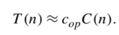
1. cop be the execution time of an algorithm’s basic operation on a particular computer,
2. C(n) be the number of times this operation needs to be executed for this algorithm.

Orders of Growth:

When comparing two algorithms that solve the same problem, if the input size is very less–

1. It is difficult to distinguish the time complexities
2. Not possible to choose efficient algorithm

2^n and the factorial function n! Both these functions grow so fast that their values become astronomically large even for rather small values of n.

The efficiencies of some algorithms may differ significantly for inputs of the same size. For such algorithms, we need to distinguish between the worst-case, average-case, and best-case efficiencies.

let us consider linear search example

SequentialSearch(A[],K)
//Searches for a given value in a given array by linear search
//Input: An array A[] and a search key K
//Output: The index of the first element in A that matches k or -1 if there are no matching elements

int i=0;
while i< n and A[i] !=k do
 i=i+1;
if i<n return i
else return -1

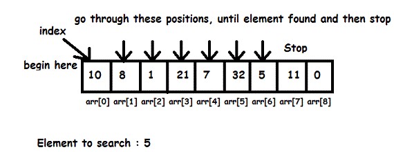
1.Worst case: No match

Analyze the algorithm to see what kind of inputs yield the largest value of the basic operation’s count C(n) among all possible inputs of size n and then compute this worst-case value.

2.Best case: Very first match

For the best-case input of size n, which is an input (or inputs) of size n for which the algorithm runs the fastest among all possible inputs of that size.

Worst-case efficiency is very important than Best-case efficiency

3.Average case: For average case efficiency assumptions are needed

The standard assumptions for linear search are that

1. The probability of a successful search is equal to p (0 ≤ p ≤ 1) and
2. The probability of the first match occurring in the ith position of the list is the same for every i.

In the case of a successful search, the probability of the first match occurring in the ith position of the list is p/n for every i. In the case of an unsuccessful search, the number of comparisons will be n with the probability of such a search being (1 -p)

1.For example, if p = 1 (the search must be successful)

1. The average number of key comparisons made by sequential search is (n + 1)/2; that is, the algorithm will inspect, on average, about half of the list’s elements.

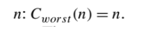
2.If p = 0 (the search must be unsuccessful)

1. The average number of key comparisons will be n because the algorithm will inspect all n elements on all such inputs.

The framework’s primary interest lies in the order of growth of the algorithm’s running time(extra memory units consumed)as its is input size goes to infinity.

Asymptotic Notations:

we are interested in, t(n) will be an algorithm’s running time( usually indicated by its basic operation countC(n), and g(n) will be some simple function to compare the count with.

1.O(big oh) Notation:

A function t(n) is said to be in O(g(n)), denoted t(n) ∈O(g(n)), if t(n) is bounded above by some constant multiple of g(n) for all large n, i.e., if there exist some positive constant c and some nonnegative integer n0 such that

big-O notation for asymptotic upper bounds

2.Ω(big omega) Notation:

A function t(n) is said to be in Ω(g(n)), denoted t(n) ∈Ω(g(n)), if t(n) is bounded below by some positive constant multiple of g(n) for all large n, i.e., if there exist some positive constant c and some nonnegative integer n0 such that

big-Ω notation for asymptotic lower bound

3.θ(big theta) Notation:

A function t(n) is said to be in θ(g(n)), denoted t(n)∈θ(g(n)), if t(n) is bounded both above and below by some positive constant multiples of g(n) for all large n, i.e.,if there exist some positive constants c1 and c2 and some non negative integer n0 such that,

big-Θ notation, an asymptotically tight bound on the running time

Non-recursive and recursive algorithms:

1.General Plan for Analyzing the Time Efficiency of Non-recursive Algorithms,

1. Decide on a parameter (or parameters) indicating an input’s size.
2. Identify the algorithm’s basic operation. (As a rule, it is located in the innermost loop.)
3. Check whether the number of times the basic operation is executed depends only on the size of an input. If it also depends on some additional property, the worst-case, average-case, and, if necessary, best-case efficiencies have to be investigated separately.
4. Set up a sum expressing the number of times the algorithm’s basic operation is executed.
5. Using standard formulas and rules of sum manipulation, either find a closed form formula for the count or, at the very least, establish its order of growth.

For example, finding Largest element in a list

MaxElement(A[])
//Determines the value of the largest element in a given array
// Input: An array A[] of real numbers
// Output: The value of the largest element in A
maxal =A[0]
for i <- 1 to n-1 do
 if A[i} >maxval
  maxval=A[i]
return maxval

1. C(n) the number of times this comparison is executed
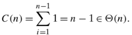
2. The algorithm makes one comparison on each execution of the loop, which is repeated for each value of the loop’s variable i within the bounds 1 and n -1, inclusive
3. Therefore, we get the following sum for C(n)

2.General Plan for Analyzing the Time Efficiency of Recursive Algorithms

1. Decide on a parameter (or parameters) indicating an input’s size.
2. Identify the algorithm’s basic operation.
3. Check whether the number of times the basic operation is executed can vary on different inputs of the same size; if it can, the worst-case, average-case, and best-case efficiencies must be investigated separately.
4. Set up a recurrence relation, with an appropriate initial condition, for the number of times the basic operation is executed.
5. Solve the recurrence or, at least, ascertain the order of growth of its solution.

For example: Factorial function

Algorithm Factorial(n)
//Computes n! recursively
//Input: a non negative integer n
//Output: The value of n!

if n=0 return 1
else return F(n-1) *n

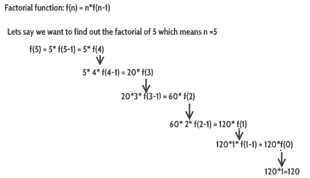
Compute the factorial function F (n) = n! for an arbitrary nonnegative integer n.

Another example of Recursive algorithm would be Towers of Hanoi.

One should be careful with recursive algorithms because their succinctness may mask their inefficiency.