Basics of an Algorithm and Different Algorithmic Approaches

Divide and Conquer:

Divide-and-conquer algorithms work according to the following general plan:

1. A problem is divided into several sub problems of the same type, ideally of about equal size.
2. The sub problems are solved (typically recursively, though sometimes a different algorithm is employed, especially when sub problems become small enough).
3. If necessary, the solutions to the sub problems are combined to get a solution to the original problem.

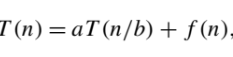
Recurrence relation for the general divide and conquer recurrence:

1. In the most typical case of divide-and-conquer a problem’s instance of size n is divided into two instances of size n/2.
2. More generally, an instance of size n can be divided into b instances of size n/b, with a of them needing to be solved. (Here, a and b are constants; a ≥ 1 and b > 1.)
3. Assuming that size n is a power of b to simplify our analysis, we get the following recurrence for the running time T (n):

The time complexity of recurrence relations is found by master theorem,

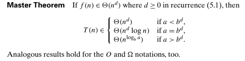
Some examples of master theorem solutions,

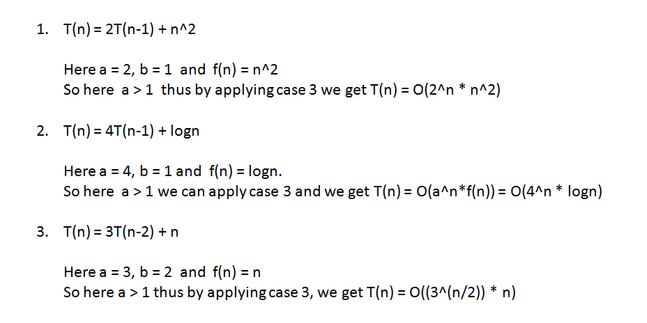
For more information,

1. https://courses.missouristate.edu/anthonyclark/325/lectures/07-master-theorem.pdf

Time complexity of below algorithms is also calculated by master theorem

1. Merge Sort
2. Quick Sort
3. Binary search
4. Multiplication of large integers

Greedy Method:

A greedy algorithm is an algorithm that constructs an object X one step at a time, at each step choosing the locally best option. In some cases, greedy algorithms construct the globally best object by repeatedly choosing the locally best option.

Greedy algorithms aim for global optimal by iteratively making a locally optimal decision. Solves problems in a Top-Down approach

Greedy algorithms have several advantages over other algorithmic approaches:

1. Simplicity: Greedy algorithms are often easier to describe and code up than other algorithms.
2. Efficiency: Greedy algorithms can often be implemented more efficiently than other algorithms.

Greedy algorithms have several drawbacks:

1. Hard to design: Once you have found the right greedy approach, designing greedy algorithms can be easy. However, finding the right approach can be hard.
2. Hard to verify: Showing a greedy algorithm is correct often requires a nuanced argument.

For example, If we have to travel from V1 to V7

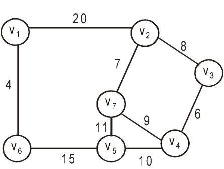
Then according to Greedy algorithm, we will consider local optimum path which will be.

1. V1 to V6 = 4
2. V6 toV5 = 15
3. V5 to V4 =10
4. V4 to V3 =6
5. V3 to V2 =8
6. V2 to V7 =7

Assemble an optimal solution to a problem

1. Making locally optimal (or greedy) choices
2. At each step, we make the choice that looks best in the current problem
3. We don’t consider results from different sub problems

When do we use Greedy Algorithms?

All the greedy problems share a common property that a local optima can eventually lead to a global minima without reconsidering the set of choices already considered.

The only problem with them is that you might come up with the correct solution but you might not be able to verify if its the correct one.

Applications of Greedy method

An application of of Greedy Algorithm is the Coin Change problem

Given currency denominations: 1, 5, 10, 25, 100, devise a method to pay amount to customer using fewest number of coins.

Our task is to use these coins to form a sum of money using the minimum (or optimal) number of coins. Also, we can assume that a particular denomination has an infinite number of coins

At each iteration, add coin of the largest value that does not take us past the amount to be paid.

Coin_Change(x,Coins[])
// Sort n coin denominations so that  c1< c2 ...
S = []
    # Iterate through coins
    for coin in denomination_list:
        # Add current coin as long as not exceeding ampoiunt
        while amount:
            if coin <= amount:
                change.append(coin)
                amount -= coin
            else:
                break
    return change

Problem reduces to coin-changing x–ck cents, which, by induction,is optimally solved by cashier’s algorithm.

It may not even lead to a feasible solution every time, as if c1 > 1: 7, 8, 9.

1. Coin change’s algorithm: 15¢ = 9 + ???.
2. Optimal: 15¢ = 7 + 8.

An application of of Greedy Algorithm is the knapsack problem

For solving the Fractional knapsack problem, we calculate the value of an item/ weight of an item ratio. Then we simply pick the best value to weight ratio items.

1. Take as much of the article with the highest value per pound (vi/wi) as possible
2. If the article with the highest value is over, take the next article with the highest value (vi/wi)
3. Continue until the sack is full

Greedy algorithms is applied in the following algorithms,

1. Prim’s algorithm
2. Kruskal’s algorithm
3. Dijkstra’s algorithm
4. Huffman trees
5. Job sequencing with deadlines/activity selection problem

For more information,

1. https://web.stanford.edu/class/archive/cs/cs161/cs161.1138/lectures/13/Small13.pdf
2. https://www2.seas.gwu.edu/~ayoussef/cs6212/greedy.html
3. https://www.cs.csustan.edu/~john/Classes/CS4440/Notes/04_GreedyAlgs/04GreedyAlgorithmsI.pdf

Dynamic Programming:

Dynamic Programming is a general approach to solving problems, much like “divide-and-conquer” is a general method, except that unlike divide-and-conquer, the sub problems will typically overlap and will not effect each other overlap.

1. Commonly used in optimization.
2. When solving sub problems, try them all, but choose the best one.

Basic Idea:

What we want to do is take our problem and somehow break it down in to a reasonable number of sub problems in such a way that we can use optimal solutions to the smaller sub problems to give us optimal solutions to the larger ones.

Unlike divide-and-conquer it is OK if our sub problems overlap, so long as there are not too many of them.

Dynamic Programming results in an efficient algorithm, if the following conditions hold:

1. The optimal solution can be produced by combining optimal solutions of subproblems;
2. The optimal solution of each subproblem can be produced by combining optimal solutions of sub-subproblems, etc;
3. The total number of subproblems arising recursively is polynomial.

Steps for Solving DP Problems

1. Define subproblems
2. Write down the recurrence that relates sub problems
3. Recognize and solve the base cases

Usually works when the obvious Divide&Conquer algorithm results in an exponential running time

Solutions for Dynamic Programming:

1. Find the recursion in the problem.
2. Top-down: store the answer for each subproblem in a table to avoid having to recompute them.
3. Bottom-up: Find the right order to evaluate the results so that partial results are available when needed.

Implementation Trick:

1. Remember (memoize) previously solved “subproblems”; e.g., in Fibonacci, we memo-ized the solutions to the subproblemsF0,F1,···,Fn−1, while unraveling the recursion.
2. if we encounter a subproblem that has already been solved, re-use solution.

Runtime≈Number of subproblems * time/subproblem

Let us take a few examples,

1.Factorial function:

Let’s take the simple example of the Fibonacci numbers: finding the n ^th Fibonacci number defined by

F_n = F_n-1 + F_n-2 and F₀ = 0, F₁ = 1

1.Recursion: The obvious way to do this is recursive, so for every time we find f(3) value three different points,

def fibonacci(n):
    if n == 0:
        return 0
    if n == 1:
        return 1

    return fibonacci(n - 1) + fibonacci(n - 2)

2.Top Down -Memoization:

The recursion does a lot of unnecessary calculations because a given Fibonacci number will be calculated multiple times. So, instead of calculating value of f(3) value three different times, we store value of f(3) in cache. So, we can easily retrieve it,

cache = {}

def fibonacci(n):
    if n == 0:
        return 0
    if n == 1:
        return 1
    if n in cache:
        return cache[n]

    cache[n] = fibonacci(n - 1) + fibonacci(n - 2)

    return cache[n]

The memoization does take extra space to store the cache values. So we compensate space complexity with time complexity.

3.Bottom-up – Iterative:

A better way to do this is to get rid of the recursion all-together by using iterative procedure, this way we don’t have to store extra values or take time to find the value.

cache = {}

def fibonacci(n):
    cache[0] = 0
    cache[1] = 1

    for i in range(2, n + 1):
        cache[i] = cache[i - 1] +  cache[i - 2]

    return cache[n]

So in terms of complexity Iterative > Memoization > Recurstion

Principle of Optimality:

A key idea is that optimization over time can often be regarded as ‘optimization in stages’. We trade off our desire to obtain the lowest possible cost at the present stage against the implication this would have for costs at future stages.

The best action minimizes the sum of the cost incurred at the current stage and the least total cost that can be incurred from all subsequent stages, consequent on this decision.

For example, If we have to travel from V1 to V7

Then according to Principle of optimality, we will consider global optimum path instead of local optimum path,

1. V1 to V2
2. V2 to V7

Applications of Dynamic method

An application of Dynamic Algorithm is the Coin change

To make change for n cents, we are going to figure out how to make change for every value x < n first. We then buildup the solution out of the solution for smaller values

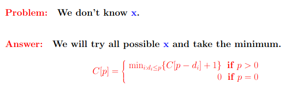
We will only concentrate on computing the number of coins.

1. Let C[p] be the minimum number of coins needed to make change for p cents.
2. Let x be the value of the first coin used in the optimal solution.
3. Then C[p] = 1 +C[p−x]

DP-Change(n)
 C[<0] =∞
 C[0] = 0
 for p= 2 t o n 
  do min =∞
   for i= 1 to k 
    do if(p≥di)
     then if(C[p−di]) + 1<min)
      thenmin=C[p−di] + 1 
      coin=i
  C[p] =min
  S[p] =coin

Instead of going for local largest coin to return at every iteration, We rather focus on minimizing the number of coins returned.

It may not leads to a feasible solution every time, as if c1 > 1: 7, 8, 9.

1. Dynamic Coin change’s algorithm: 15¢ = 7 + 8
2. Greedy Coin change’s algorithm:15¢ = 9 + ?.

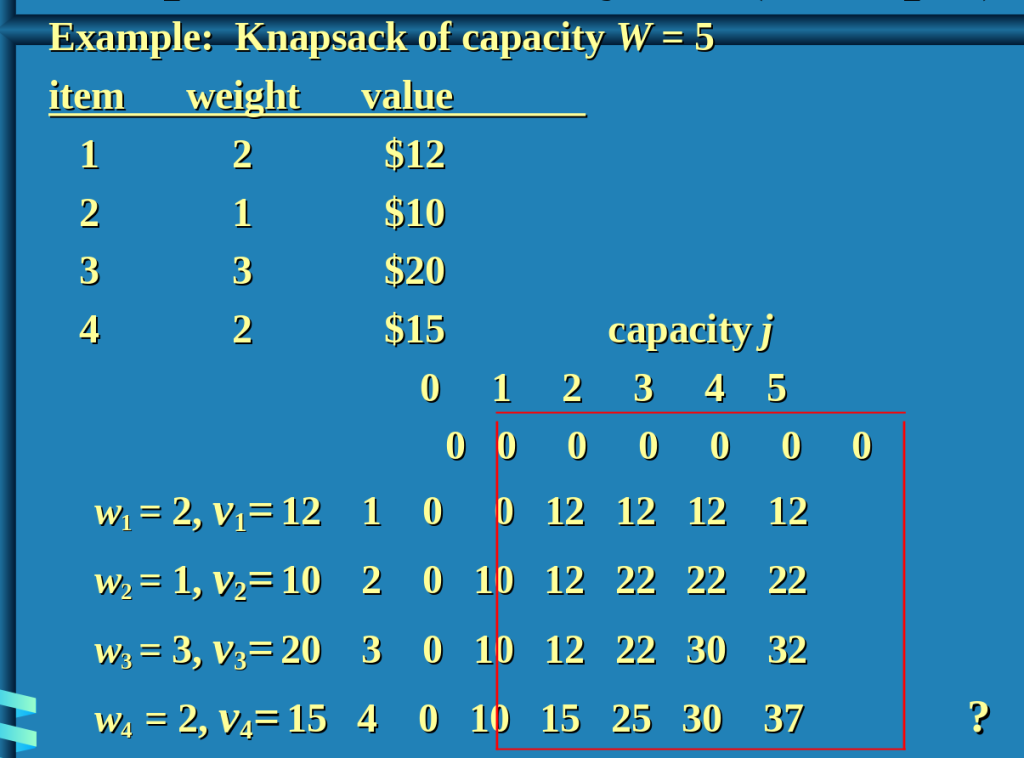
An application of Dynamic Algorithm is the knapsack problem

For solving the 0/1 knapsack problem, we calculate the value of an item/ weight of an item ratio. Then we simply check for the optimum solution from all the combination of itmes.

1. Take as much of the article with the highest value per pound (vi/wi) as possible
2. Check the maximum value/weight for all the combination of items.
3. Continue until the sack is full

Difference between Greedy algorithm and Dynamic algorithm

More applications of Dynamic programming are,

1. Warshal and Floyd Algorithm
2. Optimal Binary Search Trees
3. Traveling salesperson problem

For more information,

1. https://cs.lmu.edu/~ray/notes/dynamicprogramming/
2. https://www.youtube.com/channel/UCxX9wt5FWQUAAz4UrysqK9A
3. https://www.cs.cmu.edu/~avrim/451f09/lectures/lect1001.pdf