I attended the Vodafone session on data analysis using pandas and numpy, this blog will contain a gist of it.A basic knowledge of python would be beneficial.
“Above all else, show the data.”
Edward R. Tufte
Q.What is Data analysis?
Data Analytics is the systematic computational analysis of data or statistics, it is used for discovery, interpretation and communication of meaningful patterns in data. Also applying these patterns for decision making.

I will be using Anaconda, which is a free and open source distribution of the Python for these applications. To install and run this application, go to terminal and follow below
To install anaconda
pip install notebook
To open a jupyter notebook
jupyter notebook
A few thing to help with your python knowledge:
What is a module?
Modules in Python are simply Python files with a .py extension. The name of the module will be the name of the file. A Python module can have a set of functions, classes or variables defined and implemented. Which we can further import in another file and utilize the python definitions and statements.
What is a package?
Packages are namespaces which contain multiple packages and modules themselves. Each package in Python is a directory which must contain a special file called __init__.py. This file can be empty, and it indicates that the directory it contains is a Python package, so it can be imported the same way a module can be imported.
An Simple example of using a python module
# Area and Circumference of circle with module import

#Import module math for functions and constants
import math

#Area of the circle
r = 4
a = math.pi * (r**2)  #Use pi constant defined in math module
print(a)

#Circumference of the circle
c = 2 * math.pi * r   #Use pi constant defined in math module
print(c)
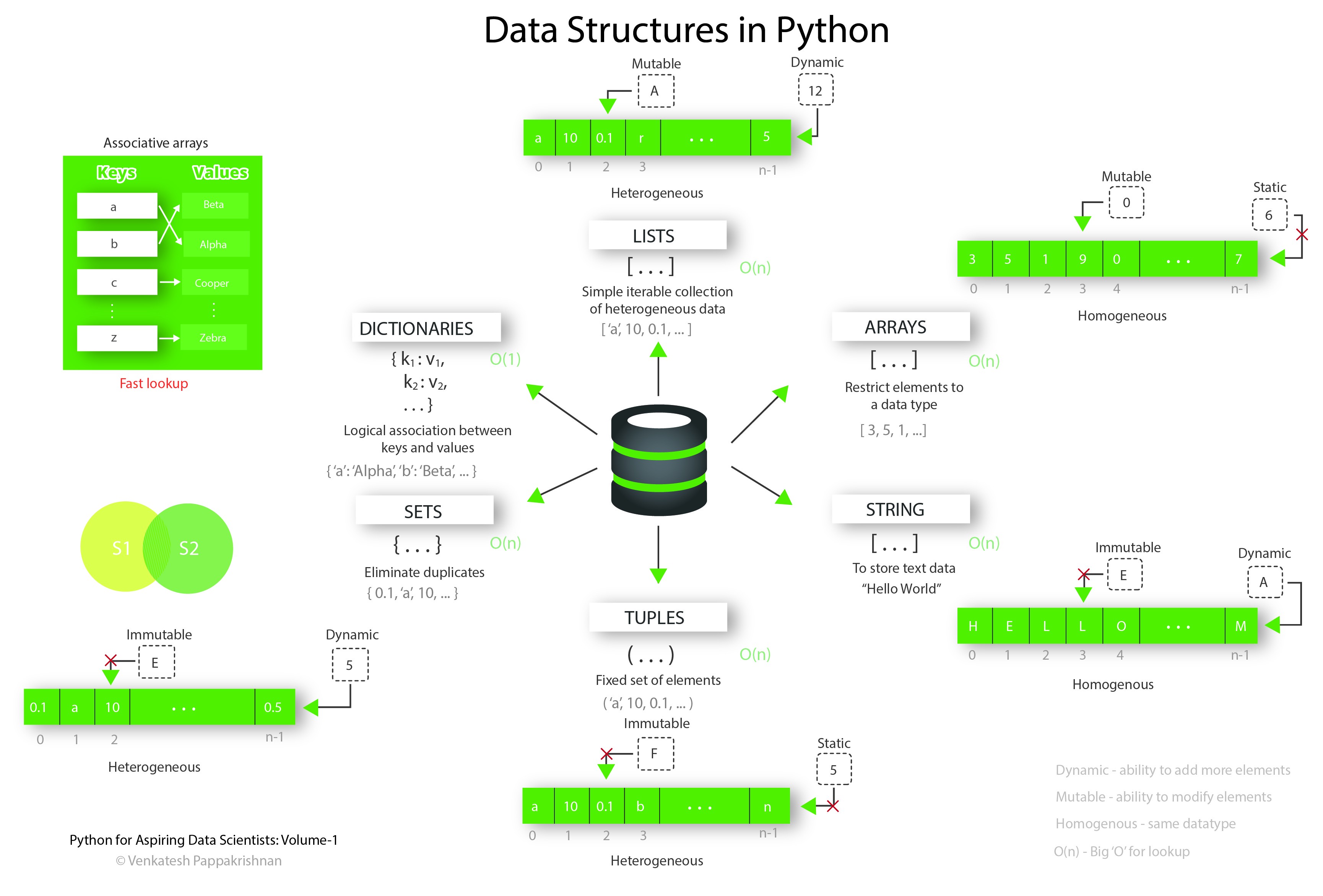
NumPy
NumPy is a python library used for working with arrays. It also has functions for working in domain of linear algebra, fourier transform, and matrices.
We use Arrays and Vectors majorly in these packages, cause manipulating a list directly is a tedious task
we can have 1 D, 2 D and 3 D array. But for simplicity, let’s take 1D.
1. How to create a NumPy array :
#Arrays
#Import Numpy module
import numpy as np
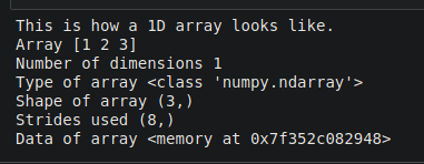
# 1D Array
print("This is how a 1D array looks like.")
one = np.array([1,2,3])
print('Array {}' .format(one))
print('Number of dimensions {}' .format(one.ndim))
print('Type of array {}' .format(type(one)))
print('Shape of array {}' .format(one.shape))
print('Strides used {}' .format(one.strides))
print('Data of array {}' .format(one.data))
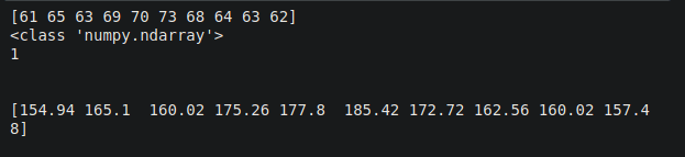
2.Converting a list into a NumPy array:
#Creating array from a list

#Consider the list of heights of baseball players
height_inches = [61,65,63,69,70,73,68,64,63,62]

#Converting this list into numpy array
height_np_inches = np.array(height_inches)
print(height_np_inches)
print(type(height_np_inches))
print(height_np_inches.ndim)
print("\n")

#Converting this array of height to cm
height_np_cm = height_np_inches * 2.54
print(height_np_cm)
3.We can find certain elements from the array
#Finding out smallest players in our players dataset
light = height_np_cm < 21
print(height_np_cm[light])
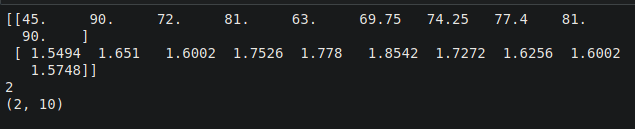
4. Making a 2 D array from lists and accessing elements
weight_pounds = [100,200,160,180,140,155,165,172,180,200]

#convert into numpy array
weight_np_pounds = np.array(weight_pounds)
weight_np_kgs = weight_np_pounds * 0.45
print(weight_np_kgs)
print("\n")

height_np_m = height_np_cm / 100
print(height_np_m)
print("\n")
#Making a 2D array from lists

baseball_total = [weight_np_kgs, height_np_m]
baseball_total_np = np.array(baseball_total)
print(baseball_total_np)
print(baseball_total_np.ndim)
print(baseball_total_np.shape)

#Looking at the players data at index 2
print(baseball_total_np[0][2],baseball_total_np[1][2])
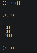
To transpose an array you need to just use array.T method or you could use np.swapaxes ( array, axis1, axis2)
#Transpose
import numpy as np
a = np.array([[2,3,4]])
print(a)
print("\n")
print(a.shape)
print("\n")
a_t = a.T
print(a_t)
print("\n")
print(a_t.shape)
5. Perform basic operations on the array:
1.mean()
print(np.mean(np_height))
2.median()
print(np.median(np_height))
3.sum()
print(np.sum(np_weight))
4.cummulative sum()
print(np.cumsum(np_weight))
5.cummulative product()
print(np.cumprod(np_weight))
6.standard deviation
print(np.std(np_weight))
7.correlation between two numpy arrays
print(np.corrcoef(baseball_np[:,0],baseball_np[:,1]))
You also have sort(), unique(), etc..
6.Can we flatten the data?
In order to get the responses to these fields like you would in Apricot Standard Reporting, you must flatten the data by creating variables. Other wise your data is given to you in a list form listing out each element of your form.
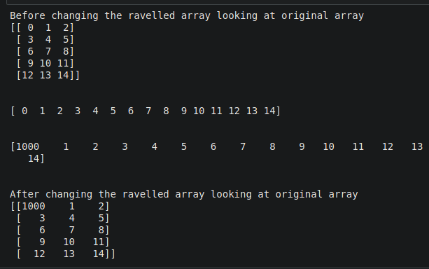
1.Ravel () function:
Return a contiguous flattened array. A 1-D array, containing the elements of the input, is returned. A copy is made only if needed.
#Ravel function for flattening of data
arr = np.arange(15).reshape((5, 3))
print("Before changing the ravelled array looking at original array")
print(arr)
print("\n")
rav1 = arr.ravel()
print(rav1)
print("\n")
rav1[0] = 1000
print(rav1)
print("\n")
print("After changing the ravelled array looking at original array")
print(arr)
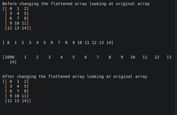
2.Flatten () Function :
Return a copy of the array collapsed into one dimension.
#Flatten function for flattening of data
arr = np.arange(15).reshape((5, 3))
print("Before changing the flattened array looking at original array")
print(arr)
print("\n")
flat1 = arr.flatten()
print(flat1)
print("\n")
flat1[0] = 1000
print(flat1)
print("\n")
print("After changing the flattened array looking at original array")
print(arr)
print("\n")
We can also concatenate or split an array or even create universal functions
7.We can also input and output data in a file
We can save into a,’npy’ file
#File Input and Output with Arrays
arr = np.arange(10)
print(arr)
print("\n")

#Saving the array into file
np.save('DA.npy', arr)

#Loading the file
np.load('DA.npy')
There are a few limitations in NumPy, hence we use Pandas
- Using “nan” in Numpy: “Nan” stands for “not a number”. It was designed to address the problem of missing values. NumPy itself supports “nan” but lack of cross-platform support within Python makes it difficult for the user.
- Require a contiguous allocation of memory: Insertion and deletion operations become costly as data is stored in contiguous memory locations as shifting it requires shifting.
Pandas
Pandas is a fast, powerful, flexible and easy to use open source data analysis and manipulation tool, built on top of the Python programming language.
In Pandas we Use Series Data Structure and DataFrame Data Structure,
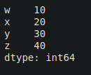
1.Series Data Structure
The Series is the one-dimensional labeled array capable of holding any data type. Series is the one-dimensional labeled array capable of carrying data of any data type like integer, string, float, python objects, etc. The axis labels are collectively called index.
In layman’s terms, Pandas Series is nothing but the column in an excel sheet.
import pandas as pd
d={'w':10,'x':20,'y':30,'z':40}
#dictionary keys act as index and values with every key act as series values
s2 = pd.Series(d)
print(s2)
2.DataFrame Data Structure
According to the Pandas library documentation, a Data Frame is a “two-dimensional, size-mutable, potentially heterogeneous tabular data structure with labelled axes (rows and columns)”.
In simple words, a Data Frame is a data structure wherein data is aligned in a tabular fashion, that is, in rows and columns
#Create Dataframe & Select columns
import numpy as np
from numpy.random import randn
np.random.seed(10)
df1=pd.DataFrame(randn(5,4),['A','B','C','D','E'],['W','X','Y','Z'])
# df1 generate random number for 5 rows and 4 columns
print(df1)
print(df1['W'])
print(df1[['W','Z']])
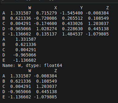
3. Data Selection and Manipulation:
1.We can select data
#DataFrame.loc() will select rows by index values
#DataFrame.iloc() will select rows by rows numbers
print(df1)
print(df1.loc['A']) # fetch particular row from dataset having index ‘A’
print(df1.iloc[3]) # fetch 3rd row from dataset
print(df1.loc[['A','C'],['X','Z']]) # fetch a subset of data from given dataset
2.We can drop data
df1.drop('A',axis=0,inplace=False)
#inplace is to True then then it will be affected in the original data structure
df1.drop('W',axis=1,inplace=False)
df1.drop('W',axis=1,inplace=True)
3. We can view the data
from numpy.random import randn
import pandas as pd
np.random.seed(101)
df2=pd.DataFrame(randn(5,4),['A','B','C','D','E'],['W','X','Y','Z'])
df2[df2>0]
df2[df2['W']>0][['Y','Z']]
df2
4.We can set and reset Index
df3=df2.reset_index() #assign natural index
df3=df2.set_index('Z') #set ‘Z’ column as index value
df4 = df3.reset_index()
df4
5.Drop missing values
import pandas as pd
import numpy as np
d={'A':[1,2,np.NaN], 'B':[1,np.NaN,np.NaN],'C':[1,2,3]}
# np.NaN is the missing element in DataFrame
df4=pd.DataFrame(d)
print(df4)

df4.dropna()         #pandas would drop any row with missing value
df4.dropna(axis=1)   #drop column with NULL value
df4.dropna(thresh=2) #Require <2 non-NA values to drop row.
6.We can group data
data = {'Company': [ 'CompA', 'CompA', 'CompB', 'CompB', 'CompC', 'CompC'],
         'Person': ['Rajesh', 'Pradeep', 'Amit', 'Rakesh', 'Suresh', 'Raj'],
         'Sales': [200, 120, 340, 124, 243, 350]}
df6=pd.DataFrame(data)
print(df6)
comp=df6.groupby("Company")             #grouping done using label name “Company”
print(comp.mean())                      #mean appliead on grouped data
comp_std=df6.groupby("Company").std()   #grouping done + standard deviation applied”
comp_std
df6.groupby("Company").max()            #group dataset based on ‘company’ label and pick maximum value in each labe
df6.groupby("Company").sum().loc["CompB"]
list(comp)
7.We can find the unique value and number of it’s occurences
df7 = pd.DataFrame({'col1':[1,2,3,4],'col2':[444,555,666,444],'col3':['abc','def','ghi','xyz']})
#col1, col2 & col3 are column labels, each column have their own values
df7
df7['col2'].unique()#fetches the unique values available in column
df7['col2'].value_counts()# count number of occurance of every value
#Type
print(type(df7['col2']))
print(type(df7[['col2']]))
8.We can also read and store data in a csv file
1.Reading from a CSV
#csv
df1 = pd.read_csv('Data/covid_19_india.csv')
df2 = pd.DataFrame({'C1' : [1, 2, 3], 'C2' : [4, 5, 6], 'C3' : [7, 8, 9]})
print(df2)
df2.to_csv('Data/new.csv')
2.Writing into a CSV
df3 = pd.read_excel('Data/Demo.xlsx',sheet_name='Sheet1')
df4 = pd.read_excel('Data/Demo.xlsx',sheet_name='Sheet2')
df5 = pd.DataFrame({'C1' : [1, 1, 1], 'C2' : [2, 2, 2], 'C3' : [3, 3, 3]})
df5.to_excel('Data/new.xlsx', sheet_name='a')
Matplotlib
Matplotlib is one of the most popular Python packages used for data visualization. It is a cross-platform library for making 2D plots from data in arrays.
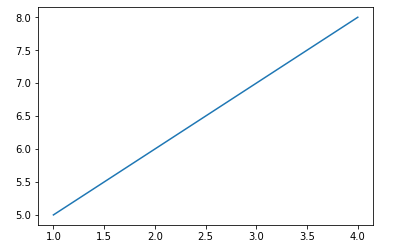
1.Plotting a basic function
#Import matplotlib functions
import matplotlib.pyplot as plt
%matplotlib inline
#Plotting function
plt.plot([1,2,3,4],[5,6,7,8])

# Function for showing what we have plotted
plt.show()
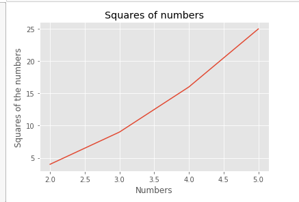
2.Plotting Quantities
#Quantities to be plotted
x = [2,3,4,5]
y = [4,9,16,25]

#Plotting function
plt.plot(x,y)

#Setting title for our plot
plt.title("Squares of numbers")

#Setting up name for x axis
plt.xlabel("Numbers")

#Setting up name for y axis
plt.ylabel("Squares of the numbers")

#Showing what we have plotted
plt.show()
3 Different Graphs
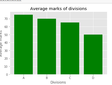
1.Bar Graph
#Bar graph

#Quantities for plotting
divisions = ["A","B","C","D"]
Avg_Marks = [75,70,65,50]

#Plotting these in the form of bar graph
plt.bar(divisions ,Avg_Marks , color = "green")

#Giving name to our plot
plt.title("Average marks of divisions")

#Naming the axes
plt.xlabel("Divisions")
plt.ylabel("Average marks")

#Showing what we have plotted
plt.show()
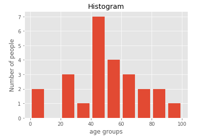
2.Histograms
#Plotting histograms

#Quantities under consideration
population_age =[22,55,62,45,21,22,34,42,42,4,2,102,95,85,55,110,120,70,65,55,111,115,
80,75,65,54,44,43,42,48]

#Defining containers aka bins of values
bins = [0,10,20,30,40,50,60,70,80,90,100]

#Plotting histogram
plt.hist(population_age, bins, histtype='bar', rwidth=0.8)

#Defining labels
plt.xlabel('age groups')
plt.ylabel('Number of people')

#Defining title for our graph
plt.title('Histogram')

#Showing the plot
plt.show()
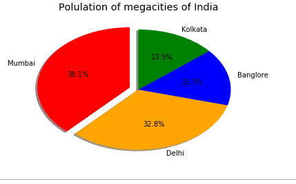
3.Pie chart
#Pie chart

#Quantities for plotting
cities = ["Mumbai","Delhi","Banglore","Kolkata"]
population = [12691836,10927986,5104047,4631392]

#Defining colors for plot
colors = ["red","orange","blue","green"]

# Plotting pie chart
plt.pie(population, labels=cities,explode = [0.1,0,0,0] ,colors=colors,autopct='%1.1f%%', shadow=True, startangle=90)

#Defining the title of our plot
plt.title("Polulation of megacities of India")

#Show what we have plotted
plt.show()
4.Box Plot
#Box plot
i = np.array([50,55,56,54,53,57,58,60,90,95,100,105])
plt.boxplot(i)
plt.show()

GitHub Repository for the following blog: https://github.com/kakabisht/data_analysis_workshop


